Time-series forecasting in finance: features, leakage, drift

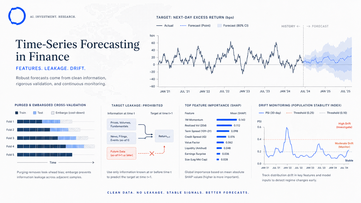
Time-series forecasting in financial markets is a discipline that fails three ways far more often than it fails the fourth. The fourth, "the model is just wrong about the future," is the one everyone worries about. The other three — feature engineering shortcuts, undetected target leakage, and silent drift — are the ones that actually break production systems.

This post is the practitioner's playbook from running the Time-Series Forecasting Quantitative Engine in production at DF Analytics. It is opinionated, technical, and focused on the failure modes that matter most for AI-native risk systems. Sections 2 and 3 in particular contain mistakes we have made ourselves and corrections we wish we had made earlier.

If you are running a forecasting model in production — ours or your own — the diagnostics at the end of each section are worth running this quarter.

10-minute read · Updated 16 May 2026

Key takeaways

• Three failure modes sink production forecasting models in finance more often than 'the model is wrong': feature engineering shortcuts, undetected target leakage, and silent drift.
• Feature engineering: lagged correctness, entity resolution, and queryable feature provenance are non-negotiable.
• Leakage: defend against look-ahead in features, look-ahead in targets, and cross-validation leakage with purged time-aware k-fold.
• Drift: monitor inputs, concepts, and performance continuously; trigger investigation on threshold crossings and feed status to the model registry.

Section 1 — Feature engineering: the boring part is the important part

The interesting model architecture choices (transformer-based vs. state-space vs. classical ARIMA-family) get most of the attention in research papers. In production, the share of model quality attributable to feature engineering is uncomfortably large — easily half, often more.

Three principles we apply:

Principle 1 — Lagged correctness is non-negotiable

Every feature must be timestamped to the moment it was available, not the moment it was generated. A fundamental data point published at 22:00 on day T is not available to a forecast made at 16:30 on day T. Treating it as available is target leakage by another name (see Section 2).

This sounds trivial. In production, feature pipelines that aggregate from multiple sources frequently mis-align timestamps. Our pipeline maintains an explicit availability timestamp per feature per observation, separate from the generation timestamp. The model is trained and inferred using availability timestamps only.

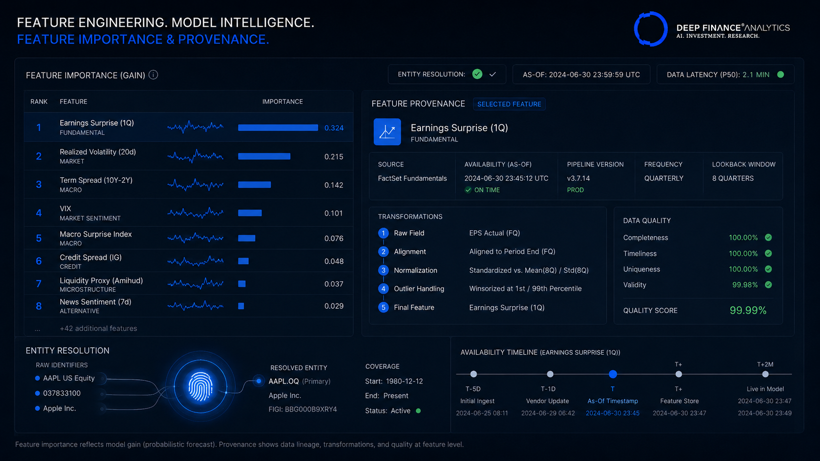
Principle 2 — Entity resolution is part of feature engineering, not before it

An issuer's ticker can change. Two issuers can share a name. A subsidiary can fall under different reporting structures over time. Entity resolution — the process of linking historic observations to the correct economic entity through corporate actions, name changes, and ownership changes — must be part of the feature pipeline.

Most issues we have seen with model performance in long-running production systems trace back to entity resolution failures introduced by a corporate action that the feature pipeline did not handle. We invest heavily in this layer; it pays off in every downstream forecast.

Principle 3 — Feature provenance must be queryable

Every feature value that enters the model has provenance: source, timestamp, pipeline version, transformations applied. This is not optional. When a downstream consumer of the forecast asks "why is the model saying this?", the answer often lives in a feature that flipped sign or magnitude two days ago. Without queryable provenance, debugging is archaeology.

Diagnostic to run this quarter: Pick five features your forecasting model uses. For each, can you produce, in under five minutes, the full provenance of the most recent value: source, availability timestamp, pipeline version, all transformations? If any of the five fails the test, the pipeline has a hole.

Section 2 — Leakage: the silent failure mode

Target leakage in time-series forecasting is the most common failure mode we have seen. It is also the hardest to detect after the fact, because leaky models look excellent in backtest and only fail in production.

Three flavours of leakage we have caught — sometimes in our own work — and how to defend against each.

Leakage flavour A — Look-ahead in features

The feature is computed using information that was not available at the prediction time. The classic example: rolling z-scores computed with the latest data point centred in the window rather than at the right edge.

The defence is the availability-timestamp discipline from Section 1. Every feature must be computable at the prediction time using only data available at that time.

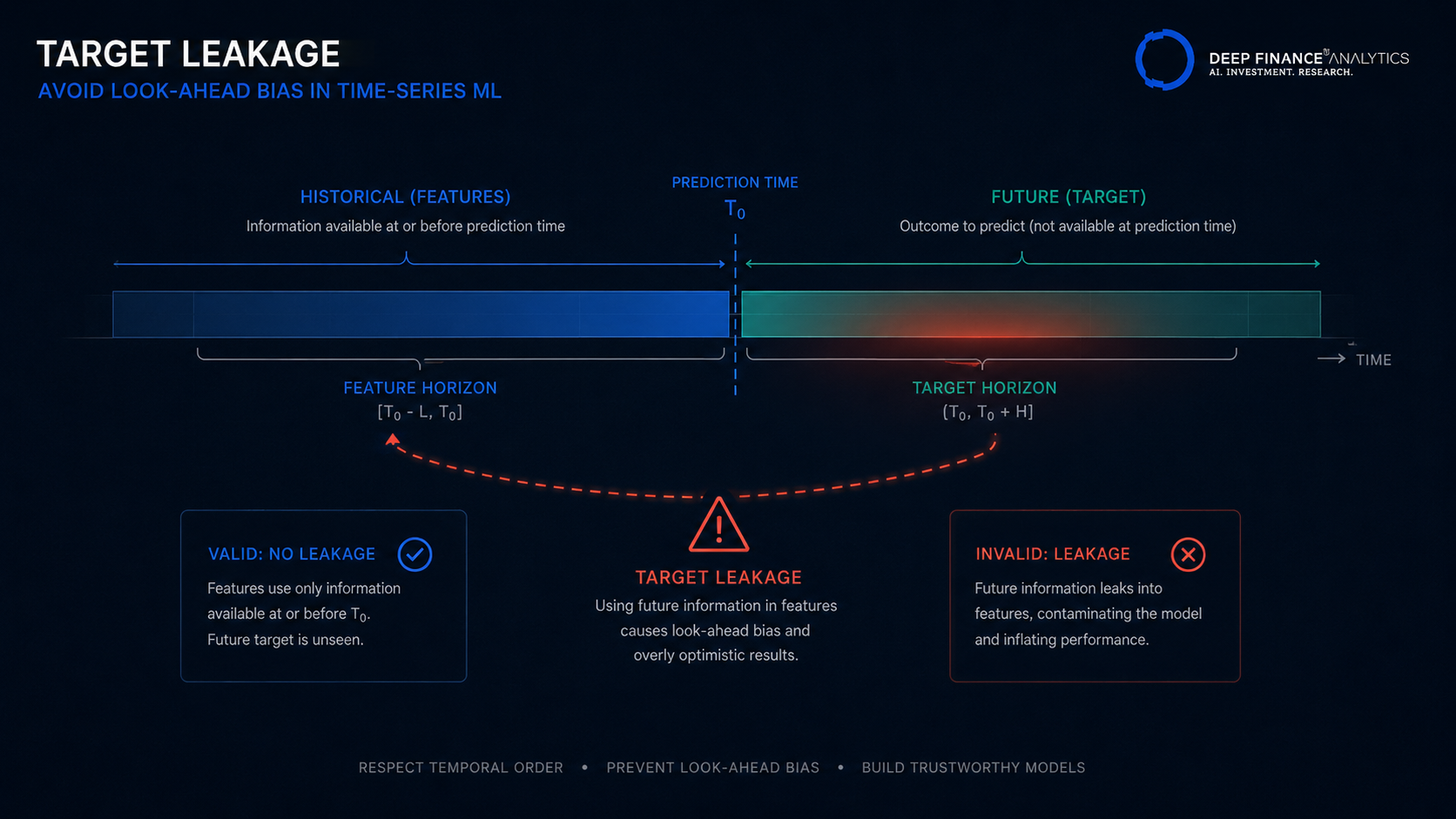
Leakage flavour B — Look-ahead in the target

The target the model is trying to predict is contaminated by information that the model could have used. The classic example: predicting next-week return from a feature that incorporates data from the days during that next week.

The defence is explicit separation of feature horizon (what the model sees) and target horizon (what it predicts). Both should be defined relative to the prediction timestamp, and the spans should never overlap.

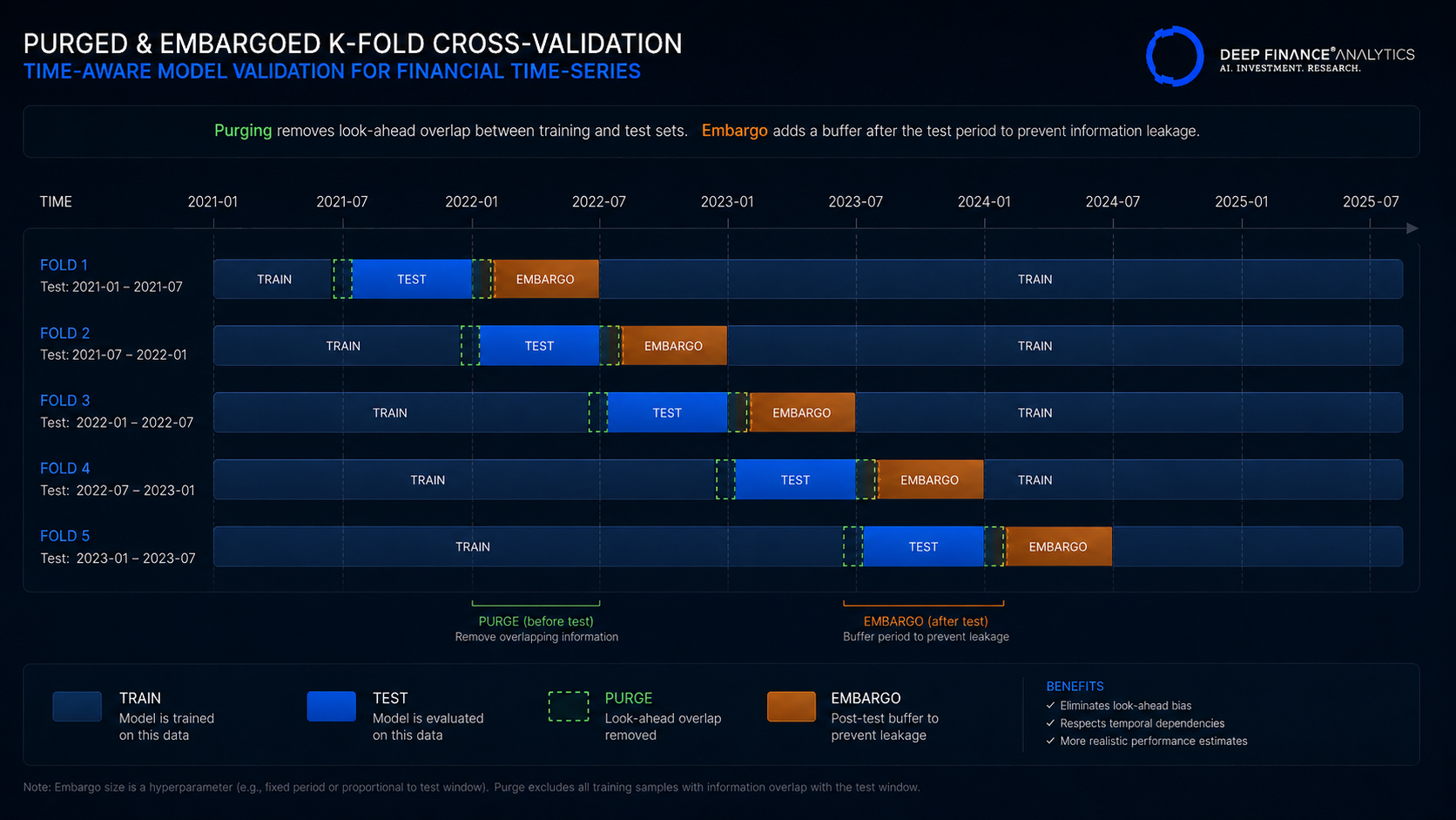
Leakage flavour C — Cross-validation leakage

Standard k-fold cross-validation on time-series data is leakage by construction: information from later periods leaks into the training set for earlier periods. The defence is purged, time-aware cross-validation: folds are sequential, and an embargo period prevents the test fold from drawing on information close in time to the training fold.

We use Lopez de Prado's purged k-fold approach for all production forecasting models. The implementation discipline is unglamorous; the alternative is models that look good in research and fail in deployment.

Diagnostic to run this quarter: Take your forecasting model and your validation pipeline. Construct a deliberately leaky version of the model (introduce one of the three flavours above). Run both through your validation. If your validation does not flag the leaky version as suspicious, your validation has a hole.

Section 3 — Drift: monitoring the world the model lives in

A forecasting model is fitted to a world that changes after the model is deployed. Drift comes in three forms, and a serious production model monitors each:

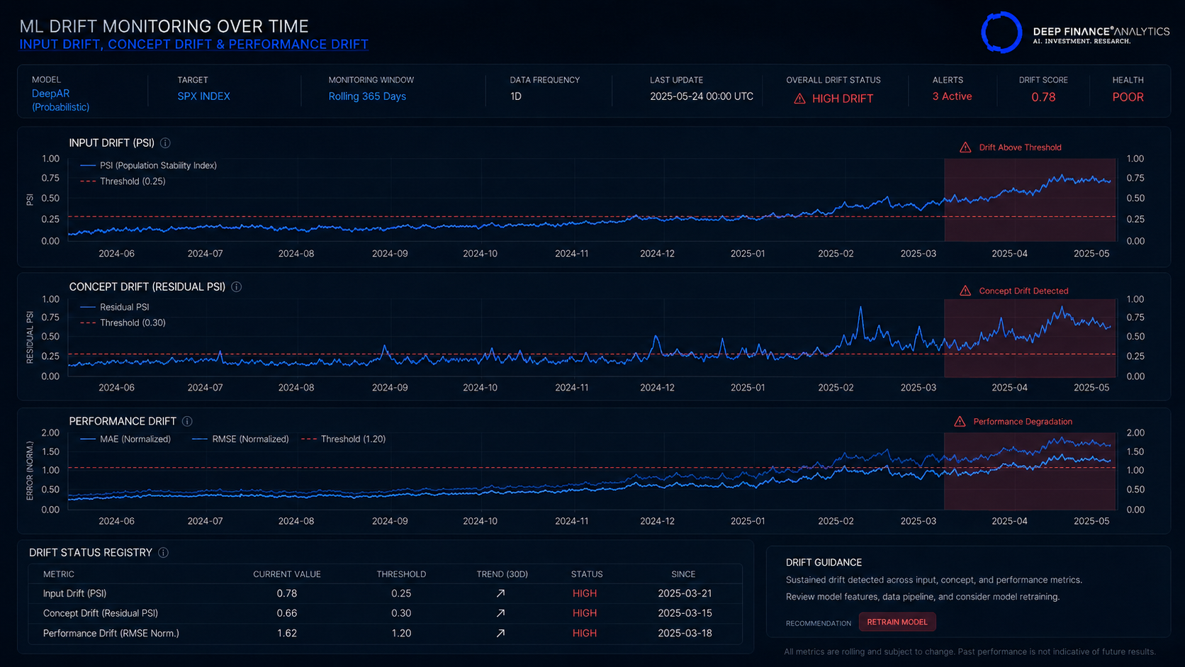
Drift type A — Input drift

The distribution of the model's inputs changes. The defence is statistical drift monitoring on every input feature — population stability indices, Kullback-Leibler divergence on binned distributions, or distribution-distance metrics depending on the feature type. Triggers fire when drift crosses a configured threshold.

Drift type B — Concept drift

The relationship between inputs and target changes, even if the inputs themselves do not. This is harder to detect; it requires monitoring the residuals of the model and looking for changes in their distribution, autocorrelation structure, or magnitude.

We track residual drift continuously and trigger investigation when the residual distribution shifts beyond a calibrated threshold.

Drift type C — Performance drift

Direct measurement of model performance against realised outcomes. The lagging metric — by definition, you can only measure performance once outcomes are known — but the most direct.

We compute rolling performance metrics on a defined cadence and trigger when they deteriorate beyond threshold.

All three types feed the model registry's drift status field. When the field changes, model owners are notified and the documentation pack reflects the new state automatically.

Diagnostic to run this quarter: For your most important production forecasting model, when was the last drift check across all three types — input, concept, performance? If the answer is more than a week ago, the drift discipline is not continuous.

A short note on architectures

Of all the things to debate, the architecture choice is the easiest to over-weight. Across our production forecasting workloads we use a mix:

• State-space models (Kalman filters, structural time-series) for univariate workloads with clear regime structure.
• Gradient-boosted decision trees for cross-sectional forecasts with rich feature sets.
• Transformer-based architectures for multi-horizon forecasts on long sequences with heterogeneous inputs.
• Hybrid models combining a classical baseline with a learned residual correction.

The choice matters; it just matters less than the three sections above. A poorly-engineered transformer will lose to a well-engineered ARIMA. The reverse is much rarer.

Where the Time-Series Forecasting Engine sits in the stack

The engine is one of the eight Quantitative Engines we ship. It is available as a REST API for OEM and white-label deployment, and it is used by PortIQ, CyronOS, and (indirectly) Epsilon through the time-series anomaly sub-score. Inside Epsilon's two-of-three coherence rule, the time-series anomaly is one of the three sub-scores that must agree before a flag is surfaced.

The engine's MRM documentation pack covers the feature pipeline, the model architecture, the validation methodology, and the drift monitoring approach. Documentation is generated continuously from runtime state, in line with the LLM-MRM template approach.

What to do this quarter

If you are running a production forecasting model and you have not run one of the diagnostics in this post, this is the week. Specifically:

• Feature provenance (end of Section 1).
• Leakage stress test (end of Section 2).
• Drift check (end of Section 3).

The three together take a few hours and they are the highest-leverage investment a forecasting team can make this quarter. If you find issues — and most teams do, the first time they run them — the fixes are typically isolated and tractable.

Coming next

19 May — Quantitative Engines: the eight APIs and when to use which. The product spotlight that walks through the full engine portfolio for OEM and white-label evaluation.

Frequently asked questions

What is target leakage in time-series forecasting?

When the model's target is contaminated by information that the model could have used to predict it. Three flavours: look-ahead in features (using data not available at prediction time), look-ahead in target (target spans information leaking back), cross-validation leakage (standard k-fold mixes future into past).

What is purged k-fold cross-validation?

A time-aware variant in which folds are sequential and an embargo period prevents the test fold from drawing on information close in time to the training fold. Lopez de Prado's purged k-fold is the standard implementation in financial time-series.

What are the three drift types to monitor?

Input drift (the distribution of model inputs changes), concept drift (the relationship between inputs and target changes), and performance drift (direct measurement of model performance against realised outcomes). Serious production models monitor all three.

How do you check for feature provenance?

Every feature value should be traceable to source, availability timestamp, pipeline version, and all transformations applied — in under five minutes. If any feature fails the test, the pipeline has a hole that will eventually cause debug archaeology.

Does architecture choice matter for forecasting?

It matters but not as much as feature engineering, leakage discipline, and drift monitoring. A poorly-engineered transformer loses to a well-engineered ARIMA. We mix state-space, gradient-boosted trees, and transformer-based architectures depending on the workload.

Related reading

• VaR vs. CVaR in stressed regimes: a 2008/2020 benchmark
• Factor models in 2026: what to keep, what to fix
• MRM documentation template for LLM-based agents

External references

• Lopez de Prado — purged k-fold cross validation
• Deep Finance Analytics — Time-Series Forecasting Engine
• Kaggle — time series forecasting best practices

About the author — Quant Research team — Deep Finance Analytics. Quant Research designs, validates, and operates the eight Quantitative Engines and the Risk Brain components. See the Insights hub for the full archive, or book a discovery call to discuss this post with the team.