Portfolio optimisation under real-world constraints

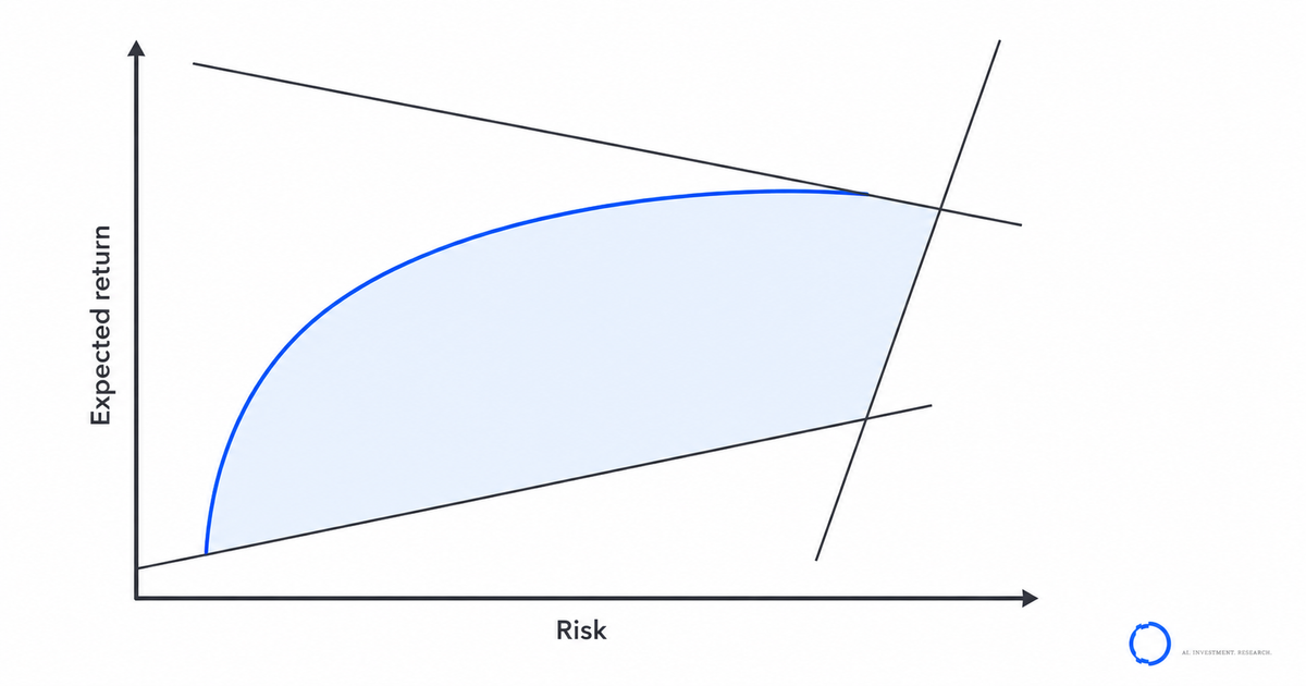
Portfolio optimisation constraints are where the elegant textbook problem quietly becomes a different problem altogether. The clean mean-variance formulation — maximise expected return for a level of variance — is a convex quadratic programme that any solver disposes of in milliseconds. Add the constraints a real mandate carries, and the same problem stops being convex, stops being unique, and in some formulations stops being solvable to a guaranteed optimum at all.

This post is the practitioner's playbook from running the Portfolio Optimisation Quantitative Engine in production at DF Analytics. It is about the gap between the optimiser you write in a notebook and the one that has to produce a tradeable, mandate-compliant, cost-aware allocation every rebalance. The interesting failures are not in the objective function; they are in the constraints and in the inputs.

If you run an optimiser in production — ours or your own — the diagnostics at the end of each section are worth running this quarter. Most teams find at least one hole the first time.

11-minute read · Updated June 23, 2026

Key takeaways

• Real mandates turn the convex mean-variance problem into a non-convex, often combinatorial one: cardinality limits, minimum lot sizes, and turnover penalties break the clean formulation.
• The constraints that actually bind — turnover, transaction costs, cardinality, group exposure caps — deserve more engineering attention than the objective function does.
• Estimation error in expected returns and the covariance matrix is the real adversary; unconstrained mean-variance amplifies it, so shrinkage, robust estimators, and hierarchical methods earn their keep.
• Treat the optimiser as a governed model: version the inputs, log the binding constraints, and make every allocation reproducible and explainable to an investment committee.

Section 1 — Why the textbook problem breaks

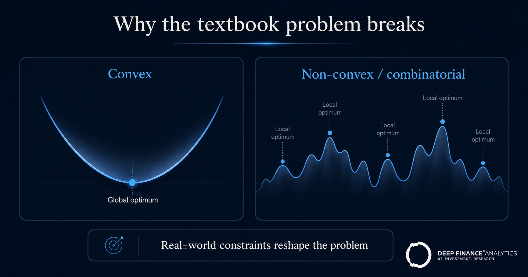
Markowitz's mean-variance formulation, now more than seventy years old, is a convex quadratic programme. Convexity is the property that makes it well-behaved: any local optimum is the global optimum, and the solver returns the same answer every time. Strip the problem down to a budget constraint and a long-only bound and it stays convex.

The trouble is that almost nothing a real mandate requires is convex. A limit on the number of holdings — a cardinality constraint — is combinatorial: you are choosing a subset of the universe, and the feasible region is no longer a smooth convex set. Minimum position sizes ("if you hold it, hold at least 50 basis points") introduce the same discontinuity from the other direction. Round-lot and minimum-trade-size rules add integrality. Each of these, on its own, moves the problem from quadratic programming into mixed-integer programming, where solve time grows sharply with universe size and a guaranteed global optimum is no longer cheap.

This is not a marginal academic point. The practitioner literature has catalogued it for years: Kolm, Tütüncü and Fabozzi's survey of six decades of portfolio optimisation frames transaction costs, real-world constraints, and input sensitivity as the practical challenges, not footnotes to the theory. The objective function is the part everyone teaches; the constraints are the part that decides whether the result is tradeable.

Operationalised: our engine separates the modelling layer (what you want to optimise) from the constraint compiler (what the mandate allows). The compiler translates a human-readable mandate — exposure caps, turnover budget, eligible universe, lot rules — into the solver's formulation, and it records which class each constraint belongs to (convex, conic, or integer) so the engineering team knows exactly when a mandate has pushed the problem into combinatorial territory.

Diagnostic to run this quarter: take your live mandate and list every constraint the optimiser enforces. For each, classify it: convex, conic, or integer/combinatorial. If you cannot say which of your constraints make the problem non-convex, you cannot reason about whether your solver is returning a true optimum or a good-enough heuristic.

Section 2 — The constraints that actually bind

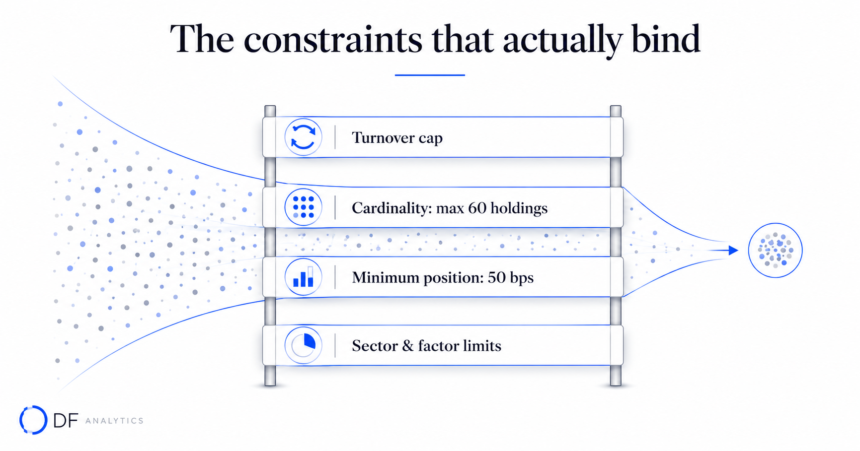
In production, a handful of constraints do most of the work — and cause most of the surprises. Three deserve dedicated engineering.

Turnover and transaction costs

An optimiser that ignores trading costs will happily propose a beautiful target allocation that is destroyed by the cost of getting there. Transaction costs belong inside the objective, not bolted on afterwards. The standard approach models cost as a function of trade size — a linear or piecewise-linear spread term plus a non-linear market-impact term that grows with the square root of participation. Because the impact term is convex, it can stay inside a well-behaved formulation; turnover limits (a hard cap on total traded notional) are linear and also tractable.

The subtlety is that cost-aware optimisation makes the problem path-dependent: the optimal portfolio depends on where you are starting from. An optimiser that does not take current holdings as an input is not cost-aware, whatever its documentation claims.

Cardinality and minimum position sizes

Investment committees rarely want a 400-name portfolio with a long tail of 3-basis-point positions. They want, say, "no more than 60 holdings, none smaller than 50 basis points." That single sentence is a cardinality constraint plus a minimum-weight constraint, and together they make the problem mixed-integer. The honest engineering answer is that for realistic universes you solve this with a combination of branch-and-bound and well-chosen heuristics, accept a small, bounded optimality gap, and report that gap rather than pretending the result is provably optimal.

Group, sector, and factor exposure limits

Most mandates cap exposure to a sector, a country, a single issuer, or a risk factor. These are linear constraints and are individually benign. The danger is interaction: a dozen reasonable caps can quietly make the feasible region empty, and a naive optimiser then fails with an opaque "infeasible" message at the worst moment. A production engine should detect which constraints conflict and surface the binding set, so a human can decide which limit to relax.

Operationalised: every allocation our engine returns ships with a binding-constraint report — the shadow prices on the constraints that were active at the optimum. This is the single most useful diagnostic an investment committee can read: it says, in effect, "here is what the mandate cost you, and here is the limit to revisit if you want more return."

Diagnostic to run this quarter: run your optimiser, then inspect which constraints were binding at the solution. If your tooling cannot tell you which limits were active and what they cost in objective terms, you are flying without the most important instrument on the panel.

Section 3 — Estimation error is the real adversary

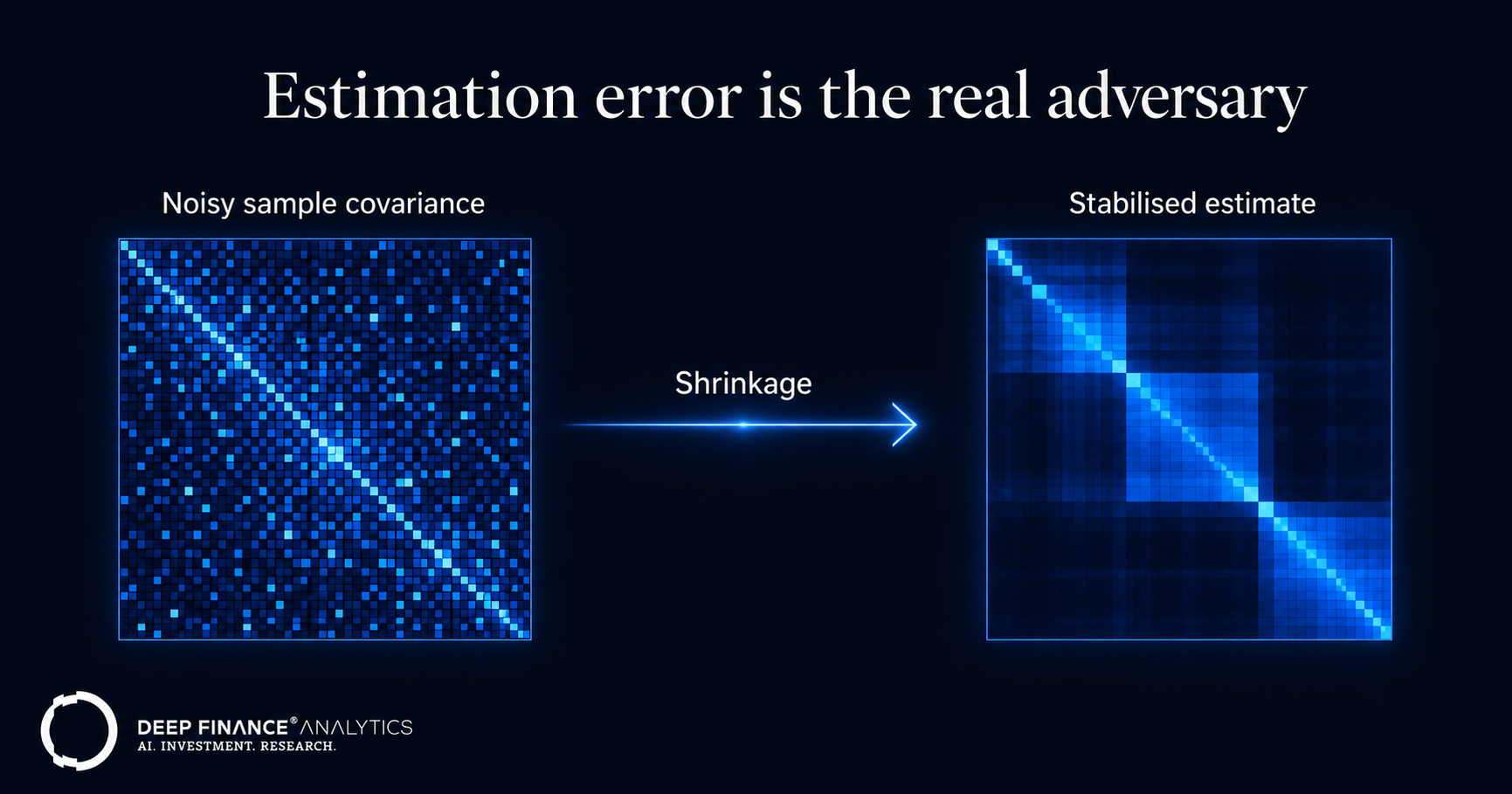
Here is the uncomfortable truth that decades of practice keep rediscovering: the largest source of bad portfolios is not a weak solver or a missing constraint. It is the inputs. Mean-variance optimisation is an error-maximising machine — it pours weight into the assets whose expected returns are most overestimated and whose risk is most underestimated, precisely because those look most attractive on paper.

Two defences matter more than any clever objective.

Tame the covariance matrix. A sample covariance matrix estimated from limited history is noisy and, for large universes, often ill-conditioned or singular. Shrinkage estimators pull the noisy sample matrix toward a structured target and dramatically improve out-of-sample stability. Factor-model covariance — decomposing risk into a small number of systematic factors plus idiosyncratic terms — does the same job structurally and ties the optimiser back to the same factor lens used elsewhere in the risk stack.

Distrust expected returns most of all. Expected-return estimates are far noisier than risk estimates, so methods that lean less on them tend to win out of sample. This is the insight behind hierarchical risk parity: López de Prado's HRP uses graph theory and clustering on the covariance matrix to build a diversified allocation without inverting that matrix and without explicit return forecasts, and his Monte Carlo experiments show it delivering lower out-of-sample variance than the classical critical-line optimiser whose own objective is minimum variance. The lesson is not "always use HRP"; it is that robustness to estimation error is a first-class design goal, not a nicety.

Operationalised: our engine treats every covariance input as a versioned, validated artifact — shrinkage intensity, factor structure, and estimation window are all logged — and it can run the same mandate through mean-variance, robust, and hierarchical formulations so the difference attributable to method (rather than to data) is visible and auditable.

Diagnostic to run this quarter: re-solve your most important mandate with the covariance estimate from a slightly different window — shift it by a month. If the resulting portfolio changes radically, your optimiser is amplifying estimation error, and a shrinkage or hierarchical approach will likely buy you stability you are currently paying for in turnover.

A short note on solvers

Solver choice matters less than the three sections above, but it is worth getting right. Pure convex problems (mean-variance with linear and conic constraints) go to a quadratic or second-order-cone solver and return provably optimal answers fast. Once cardinality and lot constraints enter, you are in mixed-integer territory, and the practical choice is between an exact branch-and-bound solver run to a bounded optimality gap and a fast heuristic that gets close without a proof. We use both, picked by problem size and the rebalance's latency budget — and we always record which path produced the result and what optimality gap it carried.

Where the Portfolio Optimisation Engine sits in the stack

The optimiser is one of the eight Quantitative Engines we ship, and it is available as a REST API for OEM and white-label deployment. It consumes risk inputs from the same covariance and factor machinery that feeds the rest of the stack, takes scenario shocks from PortIQ, and returns allocations with the binding-constraint report attached. Inside CyronOS it is the step that turns a target risk posture into a tradeable trade list.

Its model risk management documentation pack covers the objective formulation, the constraint compiler, the estimation methodology, and the solver-selection logic, generated continuously from runtime state in line with our LLM-MRM template approach. An optimiser is a model like any other: it deserves versioned inputs, logged decisions, and an audit trail an examiner could follow.

What to do this quarter

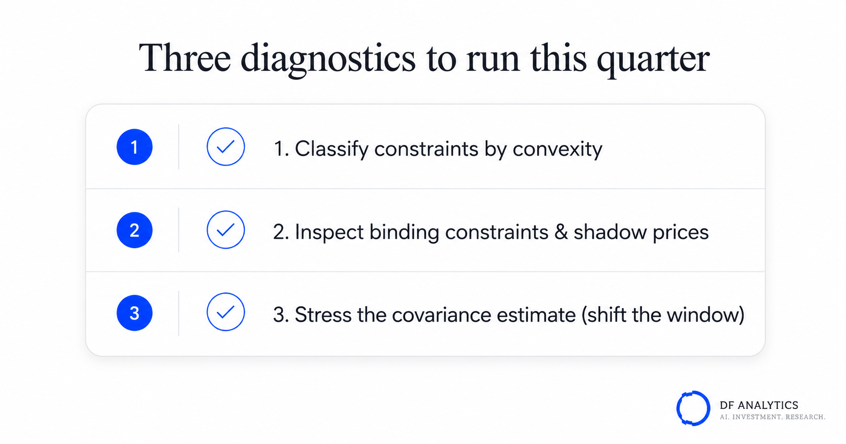
If you run a production optimiser and you have not run one of the diagnostics in this post, this is the week. Specifically: classify your constraints by convexity (end of Section 1), inspect your binding constraints and their shadow prices (end of Section 2), and stress your covariance input by shifting the estimation window (end of Section 3). The three together take an afternoon and they are the highest-leverage check a portfolio-construction team can make. The fixes, when you find issues, are usually isolated and tractable.

Coming next

30 June — Risk Heartbeat #06 — June 2026 issue. The monthly read on the regime, the flagged signals, and what the agent caught this month.

Frequently asked questions

Why are portfolio optimisation constraints non-convex?

Many real-world constraints break convexity. A cardinality constraint (a cap on the number of holdings) and minimum position sizes are combinatorial — they select a subset of assets — while round-lot and minimum-trade rules add integrality. Each turns the convex quadratic programme into a mixed-integer problem, where a guaranteed global optimum is no longer cheap to find.

Should transaction costs be inside the objective function?

Yes. An optimiser that ignores trading costs proposes targets that are uneconomic to reach. Cost is modelled as a function of trade size — a spread term plus a convex market-impact term — and added to the objective, which makes the result path-dependent: the optimal trade list depends on the current holdings.

What is the biggest source of poor optimised portfolios?

Estimation error in the inputs, not the solver. Mean-variance optimisation amplifies errors by concentrating weight in assets whose return is most overestimated and whose risk is most underestimated. Covariance shrinkage, factor-model risk, and methods that lean less on return forecasts mitigate this.

What is hierarchical risk parity?

Hierarchical risk parity (HRP), introduced by Marcos López de Prado in 2016, uses clustering and graph theory on the covariance matrix to build a diversified portfolio without inverting that matrix and without explicit expected-return inputs. In his Monte Carlo tests it produced lower out-of-sample variance than the classical critical-line optimiser.

How do you know which constraint is limiting returns?

Inspect the binding constraints at the optimum and their shadow prices. The shadow price tells you how much objective value a constraint cost — in effect, which mandate limit to revisit if you want more expected return for the same risk. A production engine should surface this report with every allocation.

Related reading

• VaR vs. CVaR in stressed regimes: a 2008/2020 benchmark
• Time-series forecasting in finance: features, leakage, drift
• Industry Risk Intelligence Platform — free sector lens

External references

• Markowitz — Portfolio Selection, Journal of Finance (1952)
• Kolm, Tütüncü & Fabozzi — 60 Years of Portfolio Optimization, EJOR (2014)
• López de Prado — Building Diversified Portfolios that Outperform Out of Sample, JPM (2016)

About the author — Quant Research team — Deep Finance Analytics. Quant Research designs, validates, and operates the eight Quantitative Engines and the Risk Brain components. See the Insights hub for the full archive, or book a discovery call to discuss this post with the team.