Factor models in 2026: what to keep, what to fix

The factor model is the workhorse of institutional portfolio risk. Forty years after Fama and French, every major risk system in production today still leans on a factor decomposition somewhere in the stack. There are excellent reasons for that: factor models are parsimonious, interpretable, well-supported by economic theory, and well-understood by regulators.

They are also — without supplementation — increasingly insufficient.

This post is a technical look at where factor models still earn their place in 2026, where they systematically under-represent risk, and how we think about layering ML and agent-driven signals on top of (not in place of) the factor view.

10-minute read · Updated 16 May 2026

Key takeaways

• Factor models still earn their place for cross-sectional decomposition, stress translation, and communication — three things they do better than alternatives.
• Three systematic failure modes: idiosyncratic residual concentration, stale loadings during regime change, and implicit stationarity in factor risk premia.
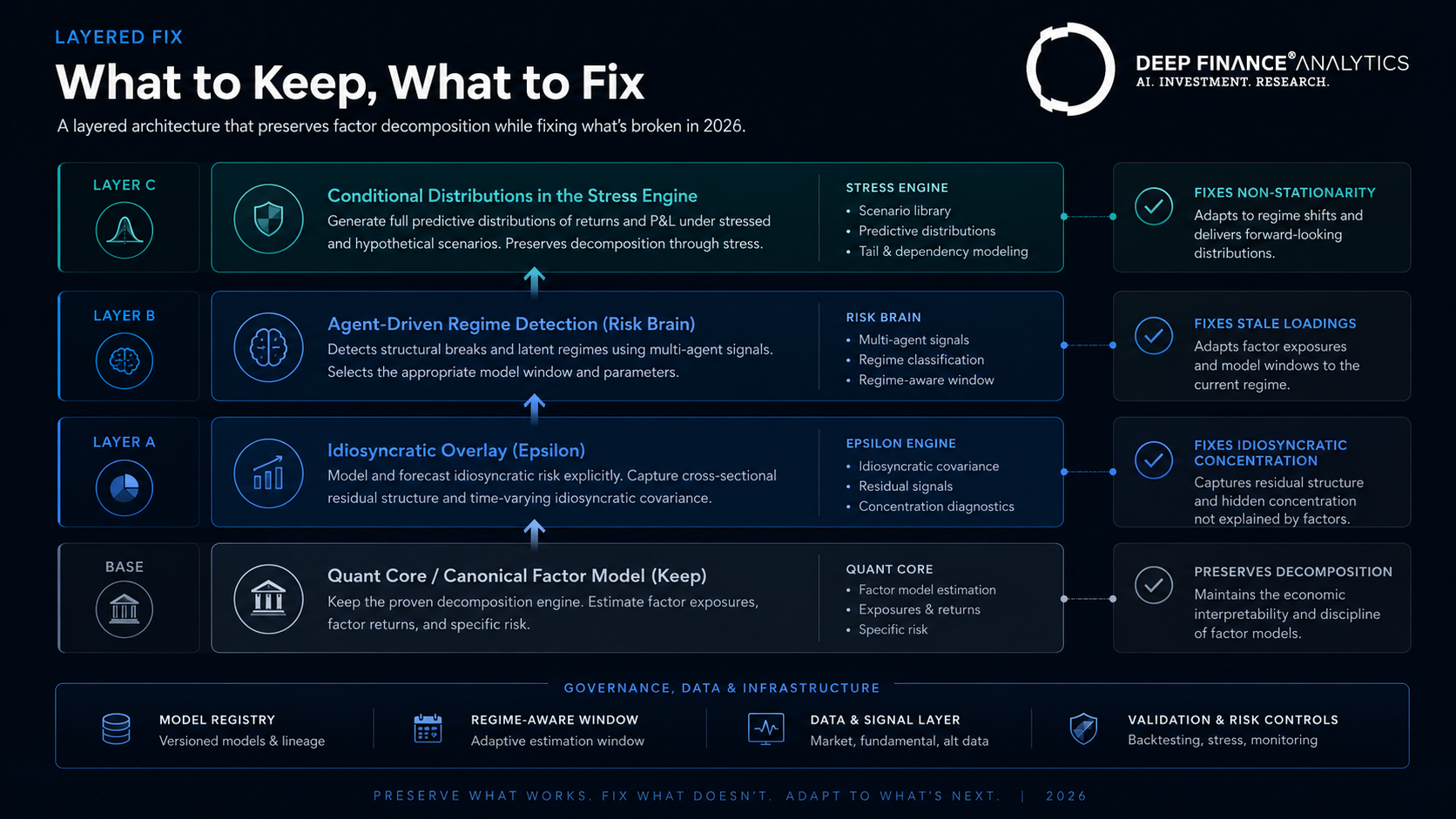
• The fix is layered: idiosyncratic overlay (Epsilon), agent-driven regime detection, and conditional factor distributions in the stress engine.
• Each layer carries its own MRM burden; documentation packs are generated continuously from runtime state rather than authored at validation cycles.

What factor models are very good at

Three things, still:

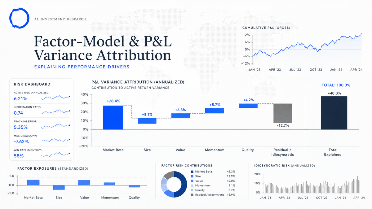
• Cross-sectional decomposition. Telling you that 73% of your equity book's daily P&L variance comes from market beta, 9% from size, 6% from value, 4% from momentum, 3% from quality, and 5% from idiosyncratic residual is exactly the kind of structured view that makes a portfolio defensible to a board or a risk committee.
• Stress translation. A coherent factor model lets you take a macro hypothesis — "rates +100bps, credit +150bps, equities −20%" — and translate it into a portfolio-level P&L. This is the substrate the narrative-to-math engine in PortIQ runs on top of.
• Communication. A factor view is legible. A board member who has not looked at quantitative risk in five years can still read a factor decomposition. That legibility is worth keeping.

We retain calibrated factor models inside CyronOS and PortIQ for these three reasons. They are not legacy; they are infrastructure.

Where factor models systematically under-represent risk

Three failure modes, each well-documented in academic literature and increasingly visible in our own client work.

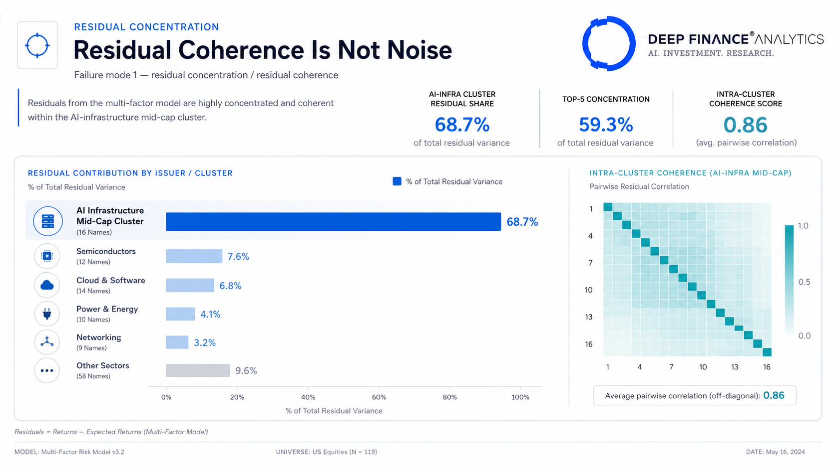
Failure mode 1 — Idiosyncratic residual concentration

A factor model treats the residual as noise. By construction the residuals across issuers should be approximately uncorrelated, mean-zero, and small enough to ignore in aggregate.

In practice, in any sector going through a structural transition, the residual is neither uncorrelated nor small. The AI-infrastructure mid-cap cluster we flagged in Risk Heartbeat #01 is a textbook example: the factor model sees fourteen separate residuals; the narrative-coherence layer sees one regime change being expressed across fourteen names. The aggregate risk is materially larger than the sum-of-residuals view suggests.

The fix is not to discard the factor model. The fix is to score residual coherence separately — which is essentially what Epsilon does — and to allow that score to feed back into the risk view.

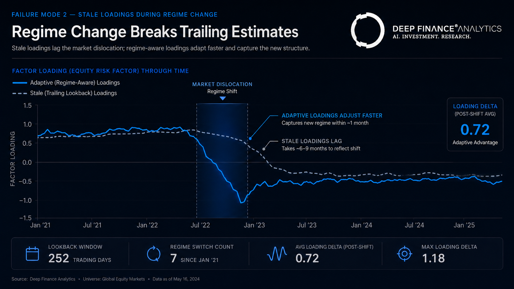
Failure mode 2 — Stale loadings during regime change

Factor loadings are estimated from historical data. When a regime changes — a sector recovers from a re-rating, a quality factor reverses sign, a momentum factor breaks down — the loadings estimated from trailing data are wrong for the new regime.

The classic example is the spring 2020 reversal of the low-volatility factor. Models calibrated on pre-COVID data treated low-vol holdings as defensive; in March 2020 they behaved like high-beta holdings because the mechanism of "defensive" had changed.

Two complementary fixes:

• Adaptive estimation windows. Rather than a fixed five-year lookback, use a regime-aware window that shortens when an agent layer detects a regime shift. This is one of the things the Risk Brain feeds back into the factor estimation pipeline.
• Challenger factor models. Maintain an alternative factor set (e.g. a learned factor space from a deep autoencoder) that runs alongside the canonical model. When the two disagree by more than a threshold, surface the disagreement as a risk signal in its own right.

Failure mode 3 — Implicit assumption of stationarity in factor returns

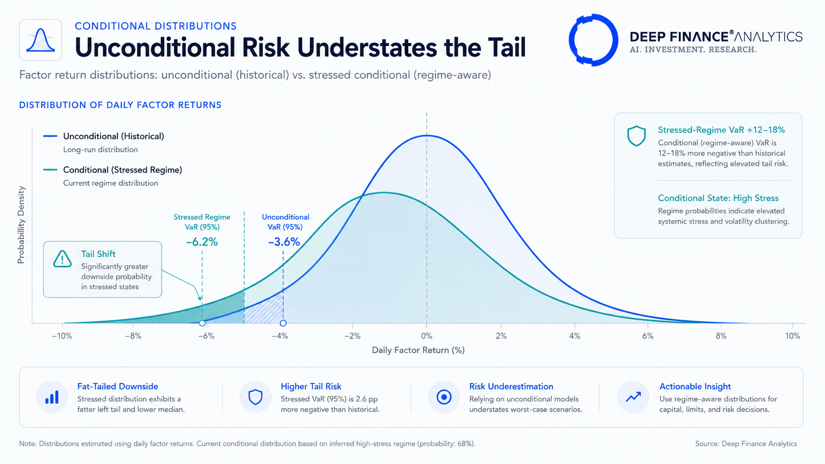
Factor risk premia are not stationary. The size premium has moved, the value premium has moved, the momentum premium has moved, and the equity risk premium itself drifts. A risk model that uses long-run factor return distributions to size factor risk understates the tail in regimes where those distributions have shifted.

The fix here is structural: use conditional factor return distributions, conditioned on observable macro and microstructure state variables. This is technical work, but the impact on tail-risk estimates is large. In our internal validation, conditional distributions produce VaR estimates that are 12–18% higher in stressed regimes than unconditional ones — and consequently survive backtesting better.

How we combine factor models with ML and agent signals

Our stack is explicit about the layering. Factor models live in the Quant Core (layer 4 in the architecture). They are calibrated, validated, and versioned in the model registry. They produce the cross-sectional decomposition that everything else hangs on.

On top of that, three things happen:

Layer A — Idiosyncratic overlay (Epsilon)

The residual is not noise. It is scored, ranked, and surfaced. Names with high idiosyncratic scores get a separate treatment in the portfolio view, in the stress engine (their residuals are not assumed to be independent during stress), and in the optimiser (constraints can be applied at the idiosyncratic-score level).

Layer B — Agent-driven regime detection

The Risk Brain monitors filings, sentiment, microstructure, and regulatory traffic. When the coherence across these signal types crosses a threshold, the factor model's estimation pipeline switches to a shorter, regime-aware window. The factor loadings are re-estimated and the new loadings flow through to the risk view.

This is the most consequential integration in the stack. It is also where the audit trail matters most: every regime switch is logged with the agent signals that triggered it, the loadings before and after, and the resulting portfolio-level risk change.

Layer C — Conditional distributions in the stress engine

Factor risk premia are estimated as conditional distributions on a small set of macro and microstructure state variables. When PortIQ runs a scenario, the relevant conditional distribution is selected based on the regime the scenario implies. A "credit crunch" scenario uses the conditional distribution of factor returns given a credit-crunch state, not the unconditional one.

The combination of these three layers preserves everything factor models do well (decomposition, stress translation, communication) and addresses what they do poorly (idiosyncratic concentration, regime change, non-stationarity).

What this means for model risk management

Each of the three layers above carries its own validation burden under SR 11-7 and the EU AI Act. Specifically:

• The factor model itself requires the standard validation: stability of loadings, out-of-sample performance, sensitivity to estimation choices.
• The idiosyncratic overlay requires validation of the composite score's calibration, false-positive and false-negative rates, and the persistence of flagged signals.
• The agent layer requires hallucination monitoring, evidence-chain completeness, and the discipline that an agent-detected regime change can only feed into model parameters via an auditable pipeline — never via an undocumented engineering change.

We ship the documentation packs for all three with PortIQ and CyronOS deployments. The pillar P5 calendar contains a follow-up post specifically on MRM documentation for LLM-driven components — coming in March.

What to do this quarter

Three practical actions that any team using factor models can take in Q1 2026:

• Audit your residual coherence. Compute, for the last twelve months, whether your residual variance across issuers in each sector has been independent or coherent. If you find clusters of coherent residuals, your factor model is under-representing the risk in those clusters.
• Run a regime-detection backtest. Construct a simple regime indicator (we use a composite of credit spread quantile, term-structure shape, and equity-vol regime) and see how your factor risk estimates would have differed if you had used regime-aware estimation windows over the last decade.
• Set up a challenger factor model. Even a simple alternative — for example, a learned factor space from an autoencoder run on the same returns — gives you a disagreement signal that is informative on its own.

None of these requires DF Analytics. They are good hygiene for any team running a factor model in 2026. If you do want to put any of them on a more rigorous footing, our quant team is happy to walk through the methodology.

Coming next

Risk Heartbeat #02 lands next Tuesday. In March we publish the governance principles essay, followed by the EU AI Act readiness checklist and the MRM template for LLM-based agents.

Frequently asked questions

Are factor models still relevant in 2026?

Yes. Factor models remain the workhorse for cross-sectional decomposition, stress translation, and board-level communication. They are necessary but not sufficient — the residual is where modern alpha and risk increasingly live.

What is residual concentration in a factor model?

Factor models treat the residual as approximately uncorrelated noise across issuers. In sectors going through structural transition, residuals are coherent — multiple issuers' residuals move together because a regime change is being expressed across many names.

What is regime-aware factor estimation?

A pattern in which the factor model's estimation window shortens when an agent layer detects a regime shift. New factor loadings are committed to the live risk view through a governed process with human-in-the-loop sign-off for material changes.

How often do regime-aware re-estimations fire?

Across our deployed PortIQ instances, on average 3–5 times per year per asset class — quieter for developed-market sovereign debt, noisier for emerging-market equities. Triggers are calibrated per asset class.

What is a challenger factor model?

An alternative factor estimation (often a learned factor space from a deep autoencoder) that runs alongside the canonical model. When the two disagree by more than a threshold, the disagreement itself becomes a surfaced risk signal.

Related reading

• Epsilon: scoring idiosyncratic risk for IC review
• VaR vs. CVaR in stressed regimes: a benchmark on 2008 and 2020
• MRM documentation for LLM-based agents: a template you can use

External references

• Fama and French — Three-Factor Model
• BIS — Conditional risk measures research
• Federal Reserve SR 11-7 — Model Risk Management

About the author — Quant Research team — Deep Finance Analytics. Quant Research designs, validates, and operates the eight Quantitative Engines and the Risk Brain components. See the Insights hub for the full archive, or book a discovery call to discuss this post with the team.